Time trajectory inference on Bone Marrow data.
This case study demonstrates the use of pseudotime trajectory inference to analyze a bone marrow dataset.
You can import the study in this tutorial with view-permission to your study list using the following link: https://cytoanalyst.tinnguyen-lab.com/studies/import/ZDdj4h49ZbA5KHXWL
Dataset
We use a subset of the bone marrow dataset from a workshop for this analysis. Below are the details of the dataset.
Dataset download link: https://export.uppmax.uu.se/naiss2023-23-3/workshops/workshop-scrnaseq/trajectory/trajectory_seurat_filtered.h5ad
Backup download:
(Please use the backup download link if the primary link becomes unavailable.)
Note: The dataset comprises 5,828 cells and has been filtered to retain only high-quality cells. Additionally, it includes precomputed embeddings and a clustering result.
For more information about the dataset, refer to the workshop
Workflow
Create a New Study
To create a new study, navigate to the Study Management page and complete the Create Study form with the following inputs:
Name:
Time trajectory inference. A descriptive name for the study.Description:
Time trajectory inference with a bone marrow dataset. A brief description of the study.
Then, click the Create Study button.
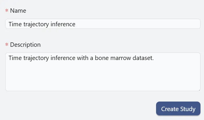
A new study will be created and added to the study table. You can use this table to manage your studies or navigate to the other pages. For more details about managing study, refer to Study Management page.

To navigate to the Data Management page for further analyses, hover over the View action of the study you just created on the study table. A pop-up will appear with options to navigate the study. Click on the Data Management option to go to the data management page.
Upload data
Uploading and processing the data
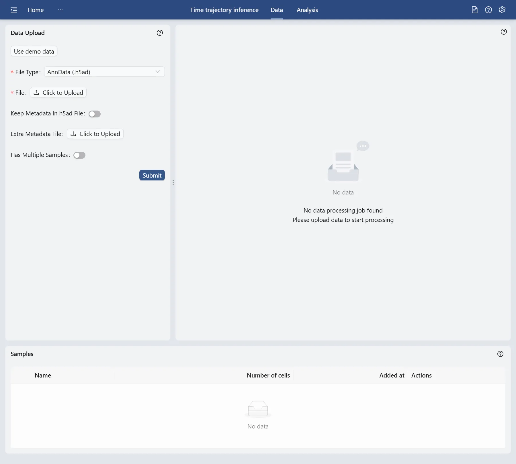
On the data management page, we will use the downloaded subset of the bone marrow dataset.
Click the Click to upload button and select the dataset to upload.
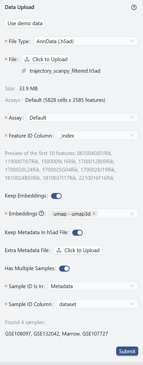
File Type:
AnnData (.h5ad). This specifies the format of the dataset file.File:
trajectory_scanpy_filtered.h5ad. The name of the dataset file.Assay:
Default. The type of assay used in the dataset. In this case, it is the default assay.Feature ID Column:
_index. The column in the dataset that contains the feature IDs. In this case, it is the gene IDs.Keep Embeddings:
True. Indicates whether to retain the precomputed embeddings in the dataset.Embeddings:
umap - umap3d. Specifies precomputed visualizations and embeddings to be kept. In this case, we select only one embedding that will be used in the further analysis.Keep Metadata in h5ad File:
True. Indicates whether to retain the metadata within the dataset file.Extra Metadata File:
Empty. An additional metadata file to be uploaded. In this case, no extra metadata file is provided.Has Multiple Samples
True. Indicates whether the dataset contains multiple samples.Sample ID Is In:
Metadata. Indicates where the sample IDs are located. In this case, they are in the metadata.Sample ID Column:
dataset. The column in the dataset that contains the sample IDs.
Finally, click the Submit button to start the data preprocessing. A job will be created in the background to process the data. Once the job is completed, the right panel will display the options for data filtering. Visit Study Logs to learn more about monitoring analysis jobs and system status.
Data Filtering
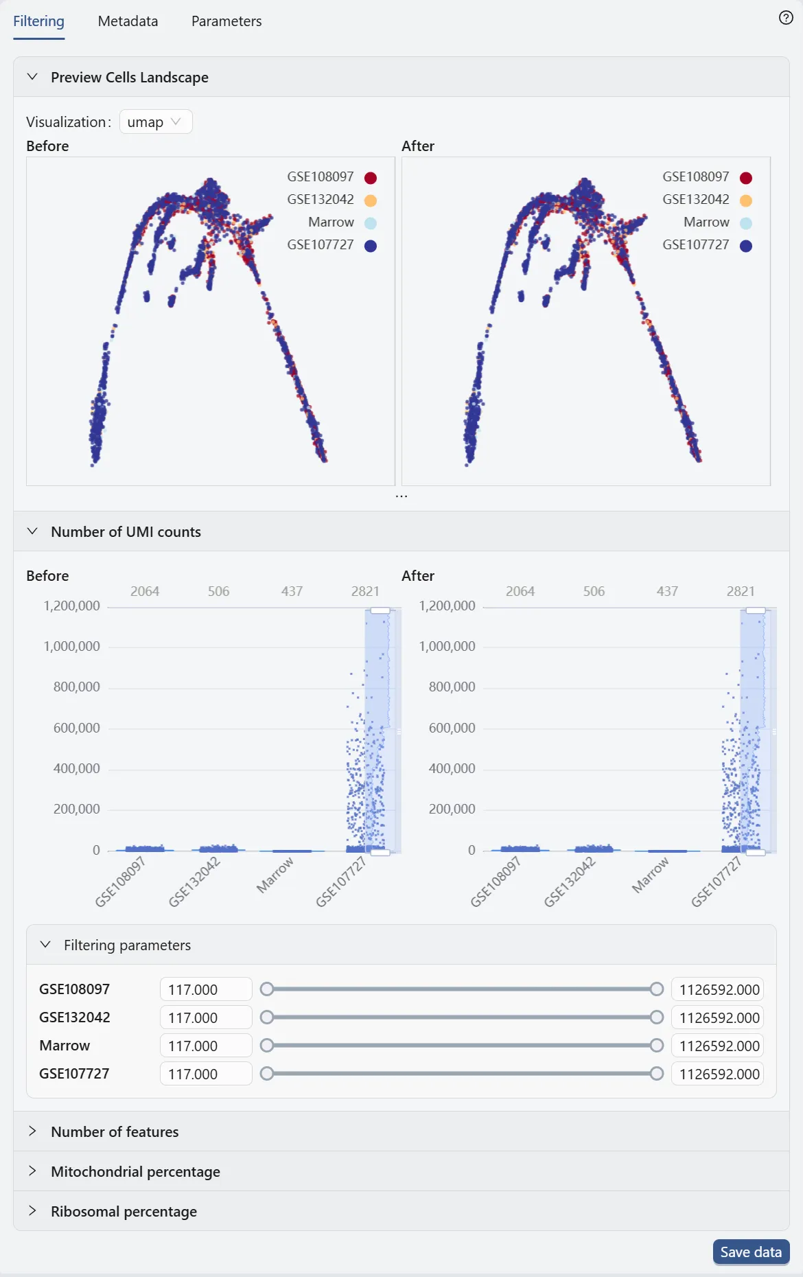
In the data filtering panel, you can filter cells based on different criteria, including the number of UMI counts, the number of genes expressed, and the percentage of mitochondrial genes.
Check out Data Management for more details on data filtering.
In this case study, we will not apply any data filtering as the downloaded dataset is already preprocessed.
Save data
Click the Save data button to open dialog for saving data.
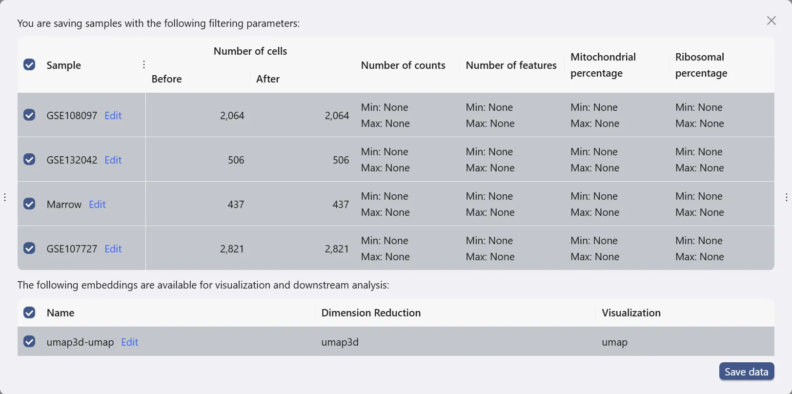
This dialog allows you to choose which samples and embeddings to save. In this case study, we will save all samples and the embedding that we chose to retain in the data uploading process.
Then, click Save data button to save the data. The newly saved data will be added to the data table.

Navigate to the Analysis page.
Once the data is saved, scroll to the top of the current page and click the Analysis to navigate to the Analysis page.
The Analysis page provides a comprehensive view of the data and analysis tools. The basic layout of the Analysis page is shown below:
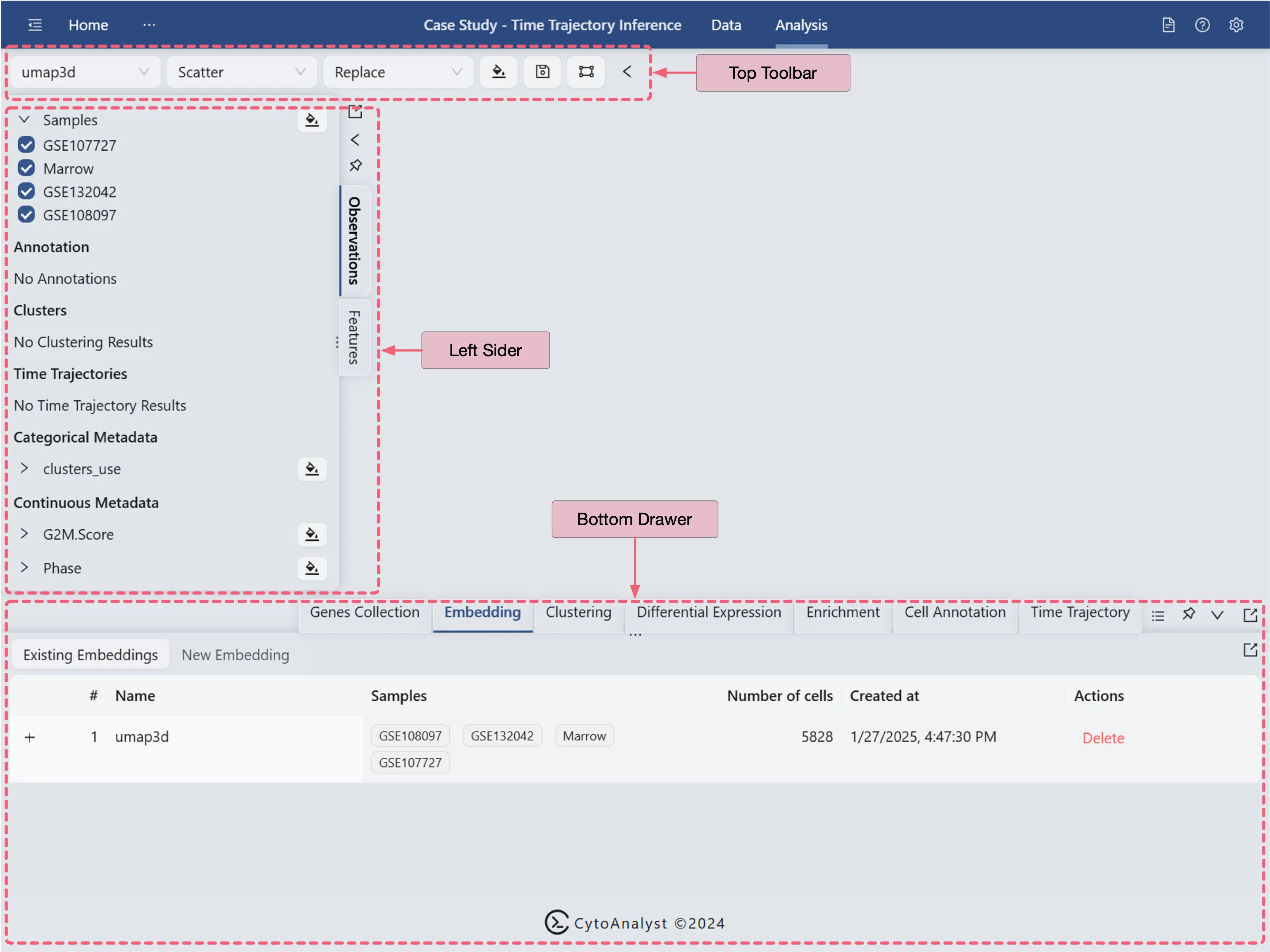
Top Toolbar: Contains dropdown menus for selecting embedding, data normalization, plot type, blending mode, and color map.
Left Sidebar: Contains the label selection panel for selecting labels to visualize.
Bottom Drawer: Contains all analysis tools
For more details about navigation and understanding the layout of the Analysis page, refer to Data Analysis.
Create a new genes collection
In this case study, we select and perform trajectory inference on the genes MS4A1, LTF, SIGLECH, and CD34, which are included in the author's list of cell-type markers.
Note: You can visit their workshop to obtain the complete list of cell-type markers collected and provided by the author.
Cell Type | Marker |
|---|---|
B cell lineage | Ms4a1 |
Granulocyte lineage | Ltf |
Dendritic cell lineage | Siglech |
HSC progenitor | Cd34 |
Follow these steps to create a gene set collection:
Click the
Genes Collectiontab on the Bottom DrawerClick the New Collection to create a new genes collection
Select Input Type as Text Input
Enter a name and the following gene sets in the text box:
Click
Savebutton to save the gene set collection.

For more details on the various methods to create a new Gene Set Collection and manage existing gene collections, refer to Gene Set Collection.
Data visualization
Visualize the cell landscape and the clustering analysis result
In this section, we will explore our data by examining the cell landscape and the result of the clustering analysis to provide an overview of the data structure.
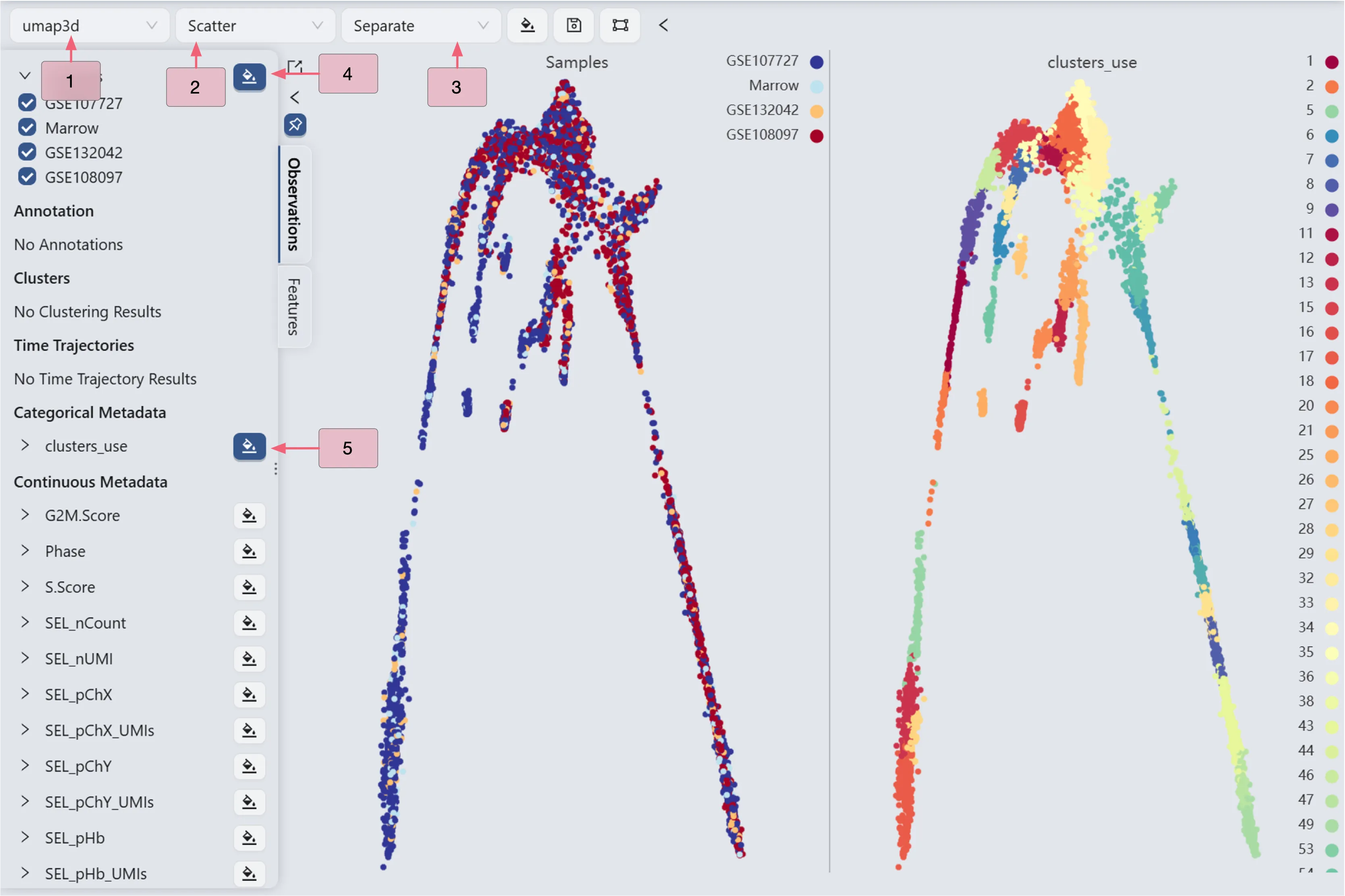
Follow these steps to visualize the cell landscape and the clustering side by side:
In the top toolbar, use the following settings:
Visualization embedding:
umap3d. Specifies which embedding will be used for visualization.Plot Type:
Scatter. Specifies the type of chart that will be displayed.Plot blending mode:
Separate. Specifies which blending mode will be used for visualization.
In the label selection panel on the left sidebar, select all samples, including GSE107727, Marrow, GSE132042, and GSE108097. Then, click the
 button next to the
 Sampleslabel to display the cell landscape. UnderCategorical Metadata, click the button next to the
 clusters_uselabel to display the clustering analysis result.
Update color mapping and other settings
Click the ![]() button on the top toolbar to update the color mapping and other settings.
button on the top toolbar to update the color mapping and other settings.

Here you will be able to:
Update the color mapping
Change the plot title
Arrange the plot by simply dragging it up or down
Change how many plots are displayed in a row
Enable and disable tooltips
Synchronize the zoom and pan across all plots
And more
For more details about data visualization, refer to Data Visualization.
Trajectory inference analysis
In this section, we will employ the Slingshot method to perform trajectory inference on the genes Ms4a1, Ltf, Siglech, and Cd34. The analysis contains following parts:
Visualize the expression of each gene.
Create and submit a new form to perform trajectory inference analyses.
Browse and visualize the results of the trajectory inference analysis.
Trajectory inference for the Ms4a1 gene.
Visualize the Ms4a1 gene expression
The Slingshot method requires specifying the starting and ending points for its parameters. Therefore, we will observe the expression of the Ms4a1 gene to manually select the starting and ending points.
Follow these steps to visualize the expression of the Ms4a1 gene and the clustering analysis result.
In the top toolbar, ensure the settings are as follows:
Visualization embedding:
umap3d. Specifies which embedding will be used for visualization.Plot Type:
Scatter. Specifies the type of chart that will be displayed.Plot blending mode:
Separate. Specifies which blending mode will be used for visualization.

Switch to the Observation tab in the left sidebar, then:
Ensure that the button next to the
Sampleslabel is unselected
Ensure that the button next to the
cluster_uselabel is selected
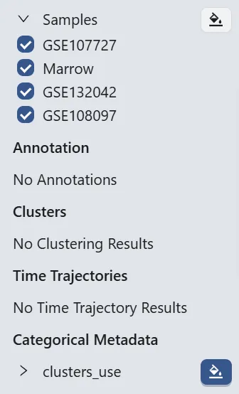
Switch to the Feature tab in the left sidebar, then:
Under
Gene set collections, you will see your created gene set collection namedCell Types Marker.Click the
B cell lineageto expand the individual genes in the gene set.Click the
 button next to the
 Ms4a1label to visualize the gene.
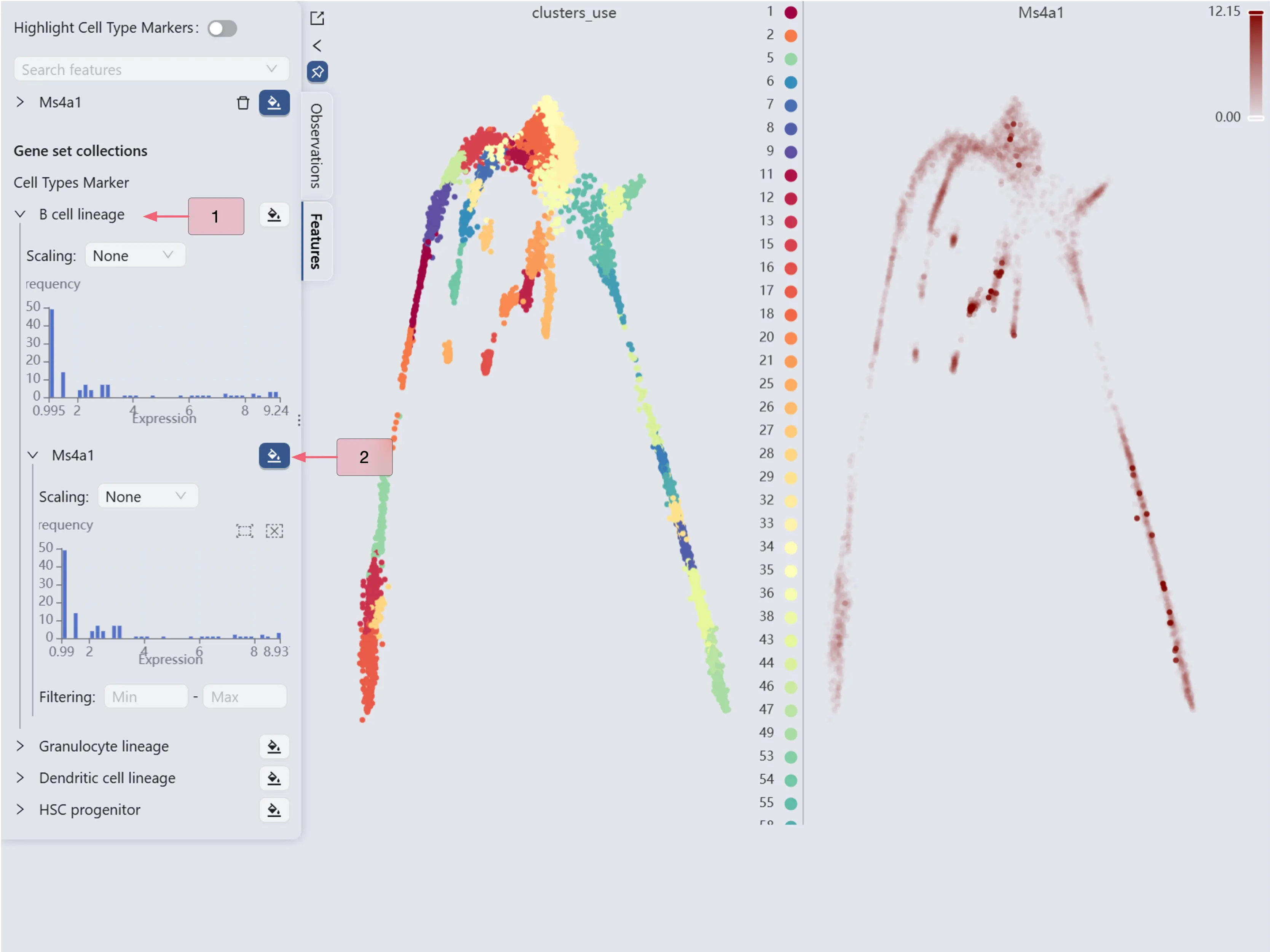
The Ms4a1 gene expression patterns (the right panel) reveal high Ms4a1 expression in cluster 20 and minimal expression in clusters 33 and 47. Based on these expression patterns, we designate cluster 20 as the starting point and clusters 33 and 47 as endpoints for the Slingshot trajectory inference parameters.
Perform trajectory inference analysis for the Ms4a1 gene
To perform trajectory inference analysis, click the Time Trajectory tab on the Bottom Drawer, and then click the New Time Trajectory button.
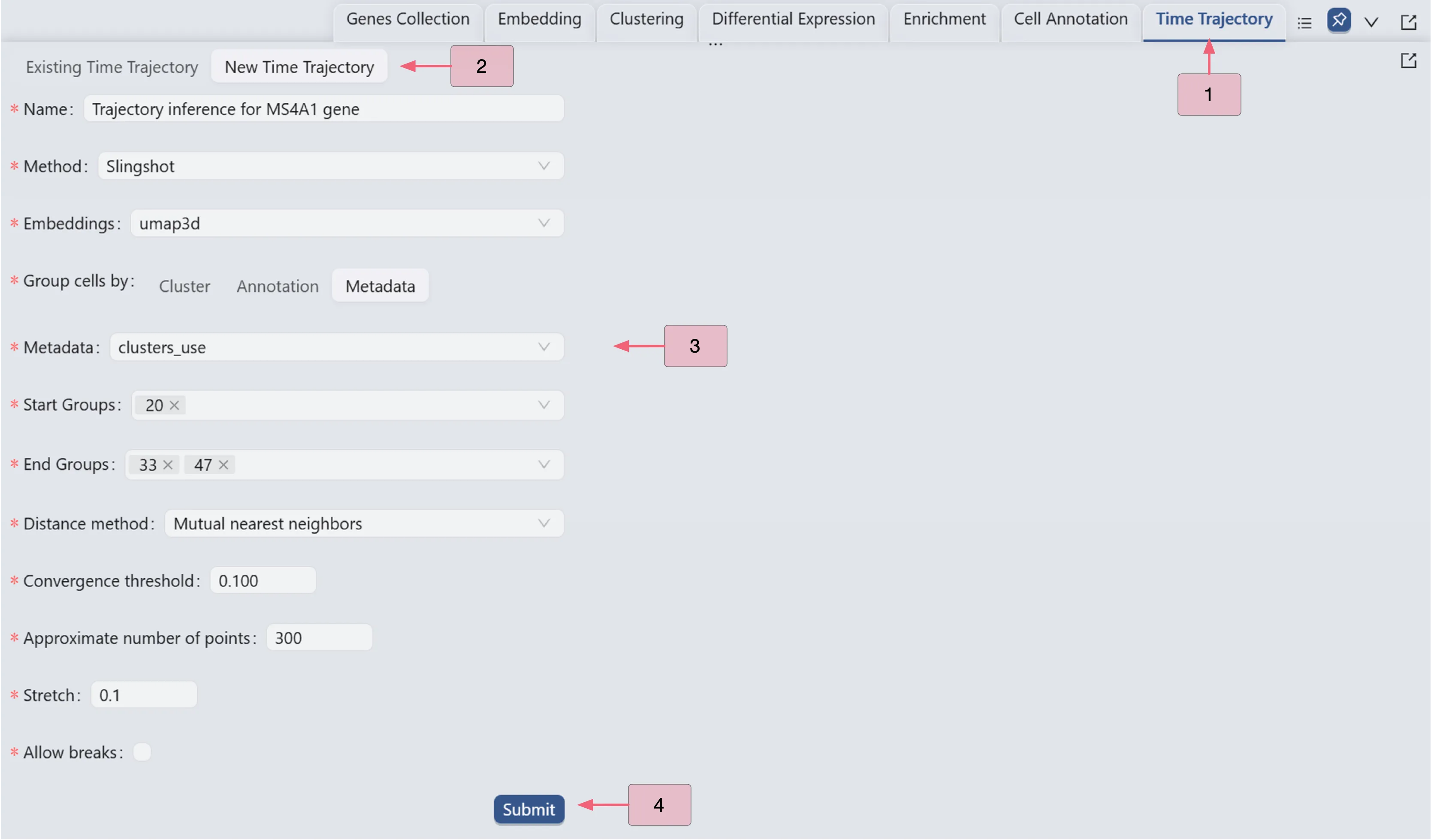
Follow these settings to perform the analysis:
Name:
Trajectory inference for MS4A1 gene. Analysis identifier.Method:
Slingshot. Trajectory inference method used for the analysis.Embeddings:
umap3d. Embedding used for the analysis. In this case, we use the generated embedding from the dataset author.Group cells by:
Metadata. Specifies cell grouping method.Metadata
cluster_use. Metadata field for cell grouping. In this case, we use the clustering analysis result from the dataset author.Start Groups:
20. Initial cluster for the trajectory inference analysis.End Groups:
33,47. Terminal clusters for the trajectory inference analysis.Distance method:
Mutual nearest neighbors. Method for computing inter-cluster distances.Convergence threshold:
0.100. Threshold for change in total distance between cells and curve projections.Approximate number of points:
300. Number of points along trajectory curves.Stretch:
0.1. Curve extrapolation factor beyond endpoints.Allow breaks:
False. Ensures continuous principal curves from origin.
Click the Submit button to create the trajectory inference analysis.
Browse and Visualize Trajectory Inference Analysis Results for the Ms4a1 gene.
Once the trajectory inference is completed, the results will be added to the Trajectory Inference Table in the Existing Time Trajectory tab. Follow these steps to view the table:
Click the
Time Trajectorytab in the Bottom Drawer.Click the
Exsiting Time Trajectorytab to switch to the existing time trajectory panel.Click the
Expand Plusicon next to the analysis name
 Trajectory inference for MS4A1 geneto expand the analysis results for theMs4a1gene.
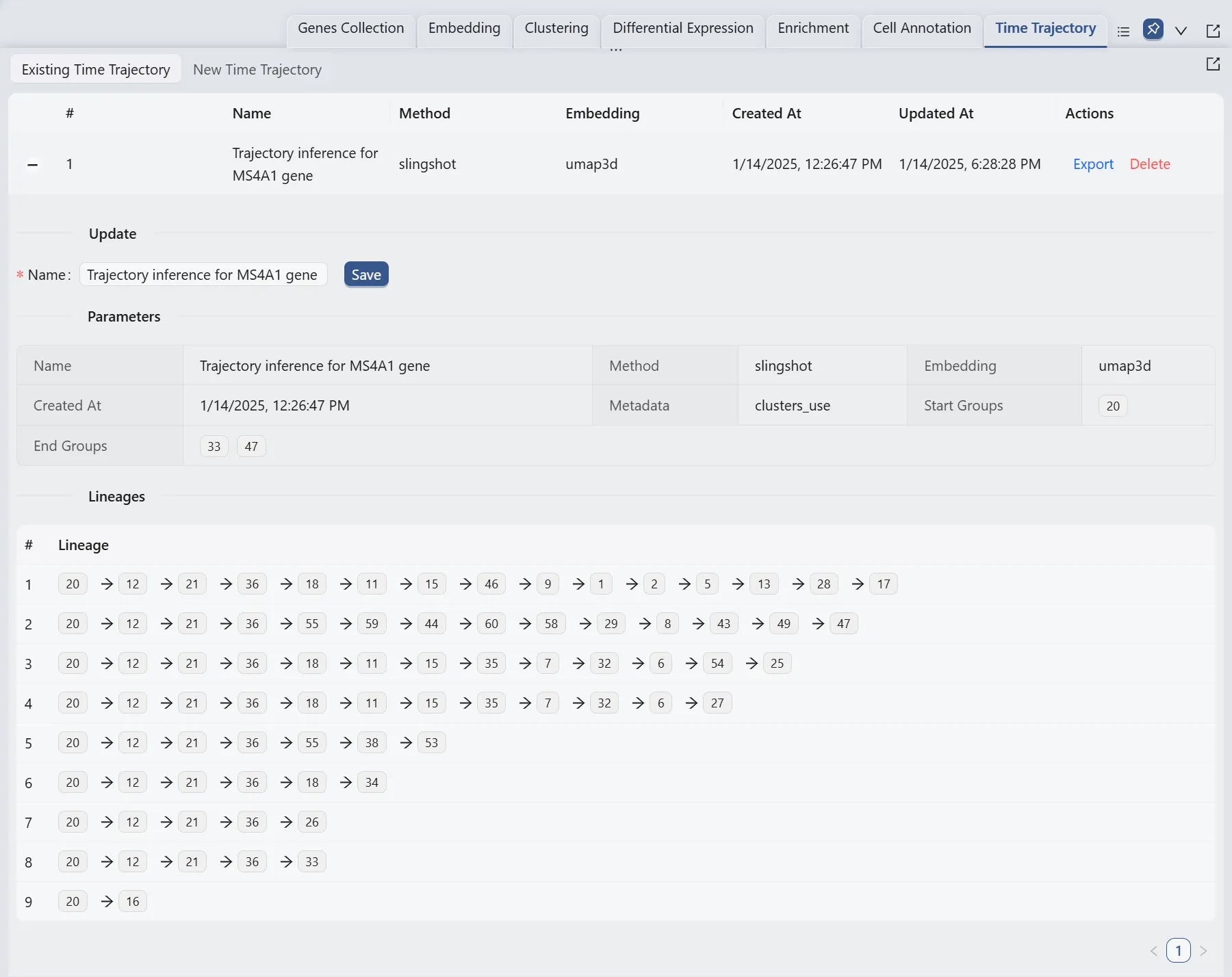
Here, we will display multiple plots to visualize the analysis results. In the top toolbar, ensure the settings are configured as follows:
Visualization embedding:
umap3d. Specifies which embedding will be used for visualization.Plot Type:
Scatter. Specifies the type of chart that will be displayed.Plot blending mode:
Separate. Specifies which blending mode will be used for visualization.

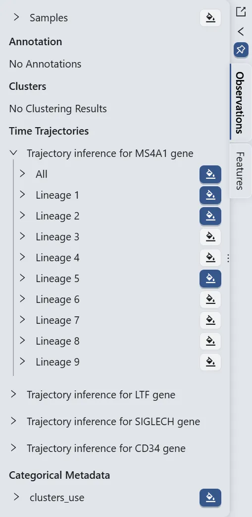
Switch to the Observeration panel in the left sidebar, then:
Click the name of the trajectory inference analysis for the
Ms4a1gene, namedTrajectory inference for MS4A1 geneto expand all results of the analysis.Click the
 button next to the
 All,Lineage 1,Lineage 2,Lineage 5labels, and ensure that the button next to thecluster_userlabel is selected
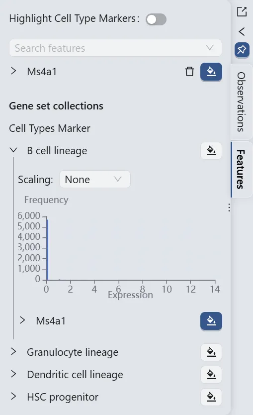
Switch to the Features panel in the left sidebar, then:
Under
Cell Types Marker, click theB cell lineageto expand the individual genes in the gene set.Ensure that the button next to the
Ms4a1label is selected.
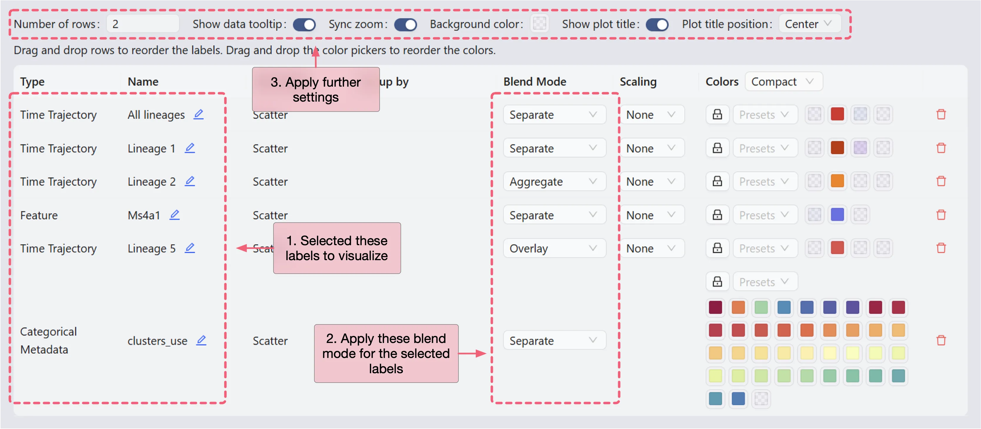
In the top toolbar, click the ![]() button to open the visualization settings panel and follow these settings:
button to open the visualization settings panel and follow these settings:
Number of rows:
2. This determines the number of rows in the grid layout.Sync zoom:
Enable. When enabled, zooming in on one scatter plot will zoom in on all scatter plots in the grid.Show plot title:
Enable. This will show the title of each plot in the grid. You can position the title to theleft,center, andright.
In the visualization settings table, focus on the key customization settings as outlined below:
Name: The name/title of the plot.
You can edit the name by clicking the
Editicon next to the current plot name.
Blend Mode: The blending mode used in the plot. Blend mode can be used to combine multiple plots into one visualization. See Blend Mode for details how to use blending modes.
Color: The color mapping used in the plot. Depending on the chart type, the color mapping can be of two types:
Value: The color mapping is based on the expression values, such as the minimum and maximum expression values.Group: The color mapping is based on the groupings, such as the metadata, clusters, or annotations.
For more details about color customization, refer to Visualization Settings.
Action:
Click the
Removeicon to remove the plot from the grid if needed.
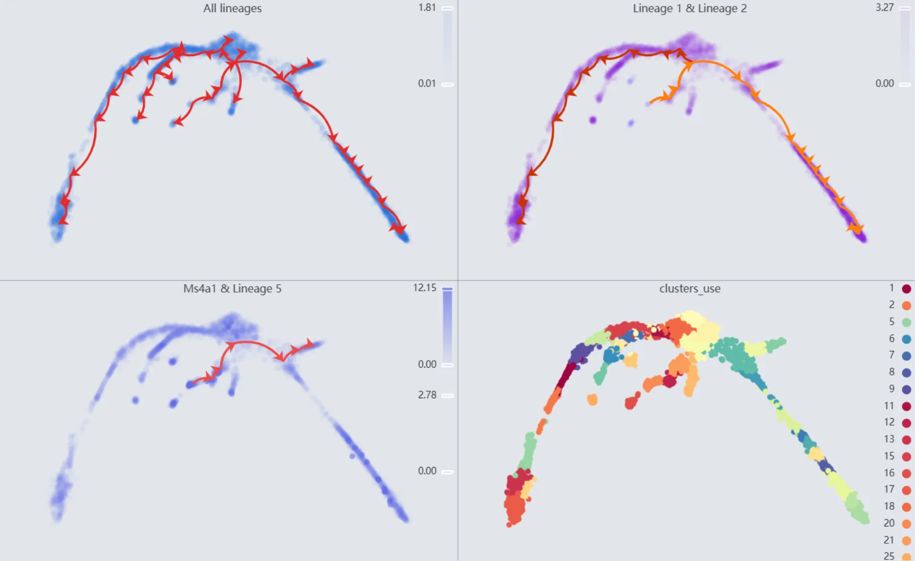
Click anywhere outside the visualization settings panel to close it. The details of all the plots are:
First plot:
All lineages. Displays the complete trajectory lineage map of the analysis.Second plot:
Lineage 1 & Lineage 2. Shows the developmental pathways from the starting to the ending groups.Third plot:
Ms4a1 & Lineage 5. Illustrates theMs4a1gene expression overlay with the representative lineageLineage 5.Fourth plot:
clusters_use. Shows the original clustering result that helped determine the starting and the ending groups.
Trajectory inference for the Ltf gene
Visualize the Ltf gene expression
We will observe the expression of the Ltf gene to manually select the starting and ending points for the Slingshot method parameters.
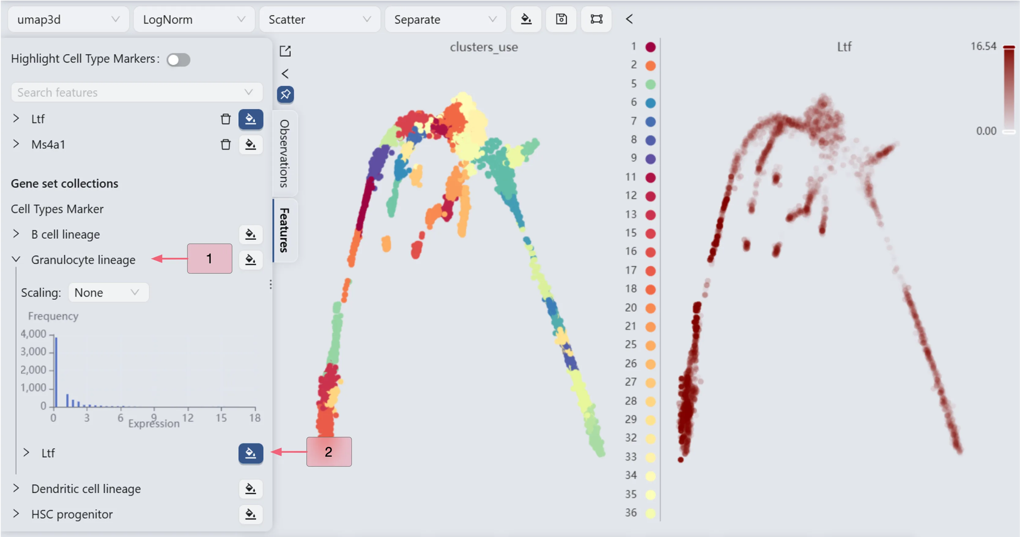
The Ltf gene expression patterns (the right panel) reveal high Ltf expression in cluster 5 and minimal expression in clusters 9 and 17. Based on these expression patterns, we designate cluster 5 as the starting point and clusters 9 and 17 as endpoints for the Slingshot trajectory inference parameters.
Perform trajectory inference analysis for the Ltf gene
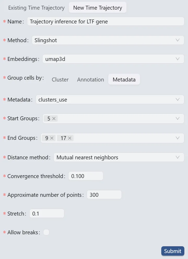
Follow these settings to perform the analysis:
Name:
Trajectory inference for LTF gene. Analysis identifier.Method:
Slingshot. Trajectory inference method used for the analysis.Embeddings:
umap3d. Embedding used for the analysis. In this case, we use the generated embedding from the dataset author.Group cells by:
Metadata. Specifies cell grouping method.Metadata
cluster_use. Metadata field for cell grouping. In this case, we use the clustering analysis result from the dataset author.Start Groups:
5. Initial cluster for the trajectory inference analysis.End Groups:
9,17. Terminal clusters for the trajectory inference analysis.Distance method:
Mutual nearest neighbors. Method for computing inter-cluster distances.Convergence threshold:
0.100. Threshold for change in total distance between cells and curve projections.Approximate number of points:
300. Number of points along trajectory curves.Stretch:
0.1. Curve extrapolation factor beyond endpoints.Allow breaks:
False. Ensures continuous principal curves from origin.
Click the Submit button to create the trajectory inference analysis.
Browse and Visualize Trajectory Inference Analysis Results for the Ltf gene
Once the trajectory inference is completed, the results will be added to the Trajectory Inference Table in the Existing Time Trajectory tab.
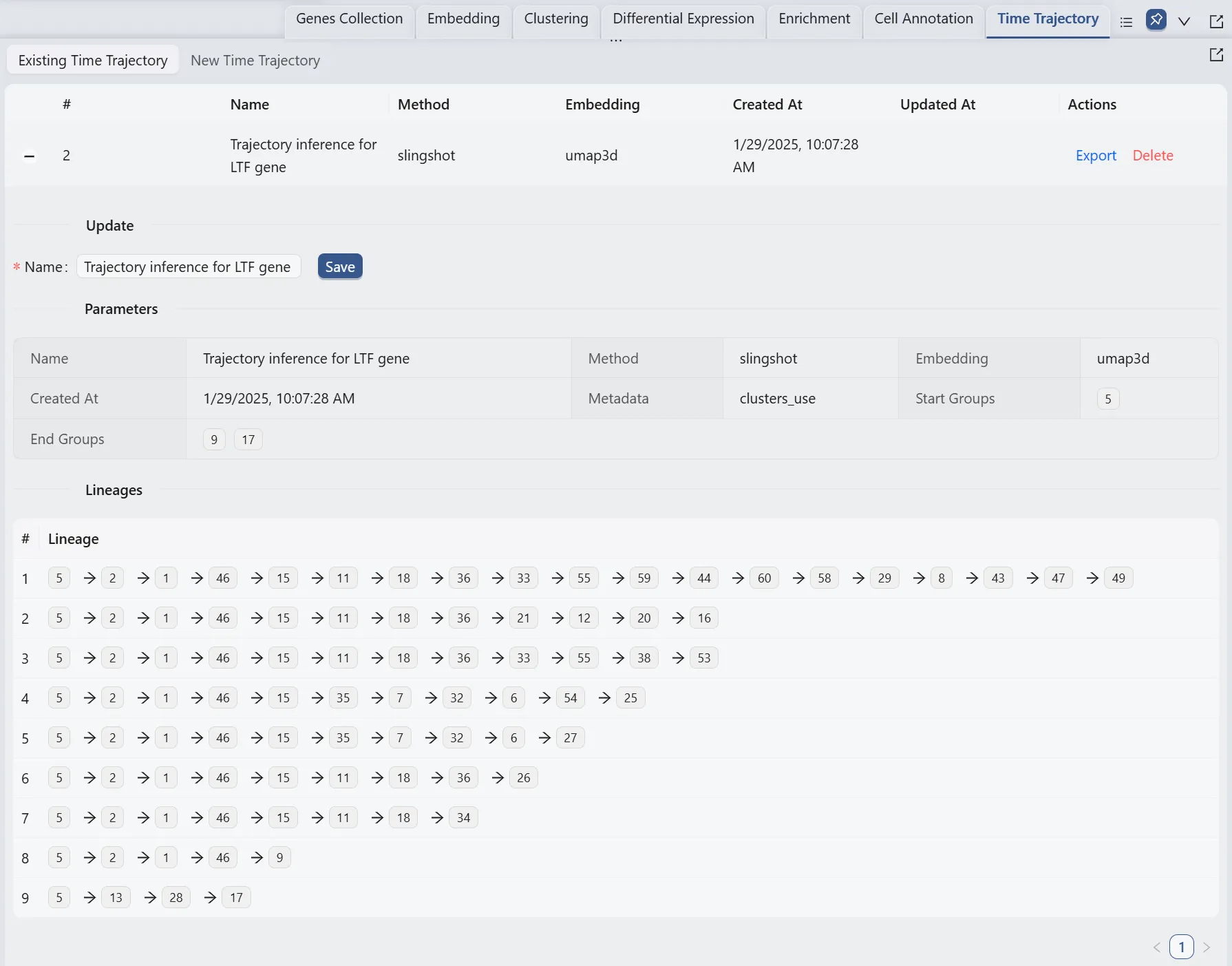
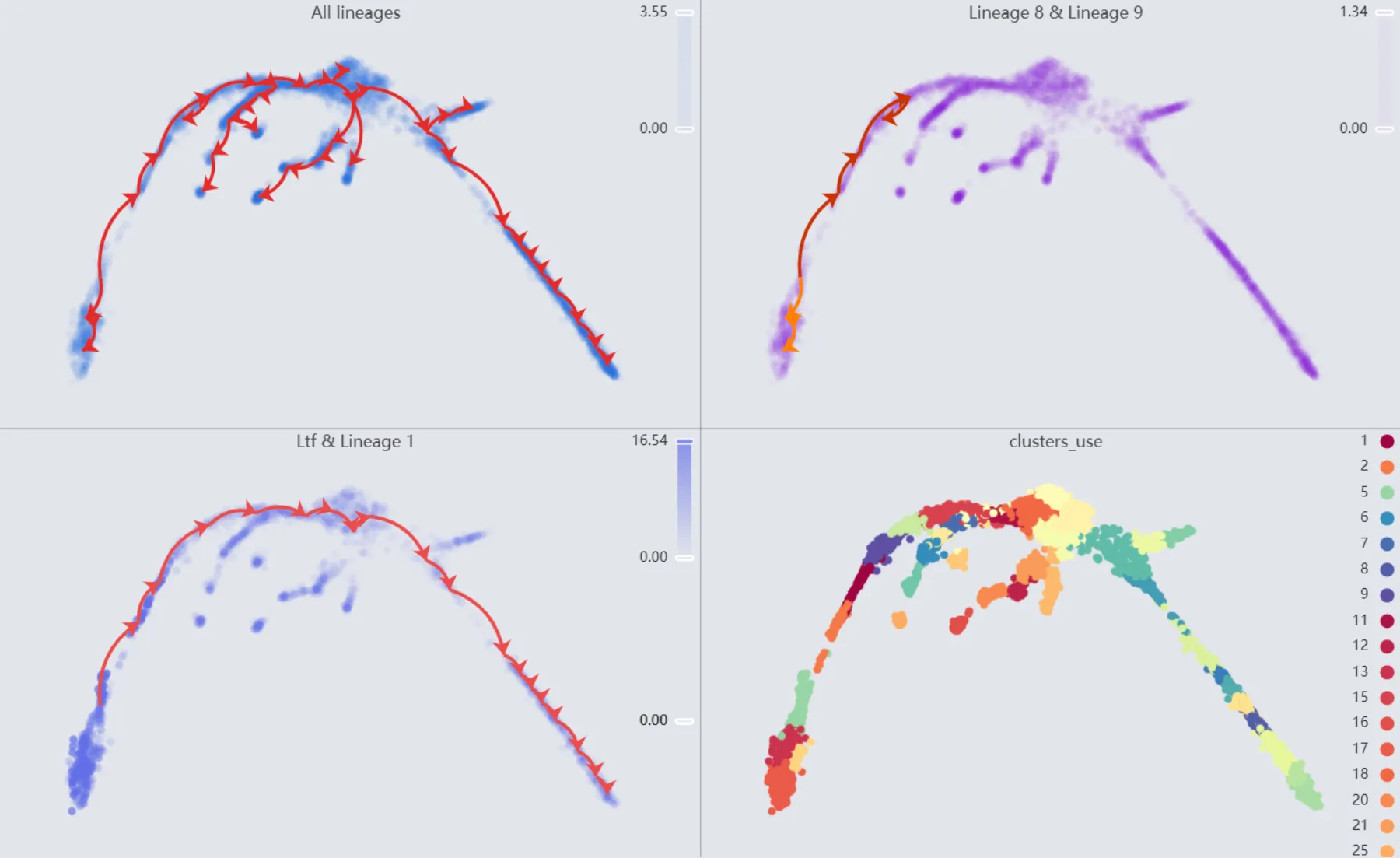
Also, we will display multiple plots to visualize the analysis results. The details of all the plots are:
First plot:
All lineages. Displays the complete trajectory lineage map of the analysis.Second plot:
Lineage 8 & Lineage 9. Shows the developmental pathways from the starting to the ending groups.Third plot:
Ltf & Lineage 1. Illustrates theLtfgene expression overlay with the representative lineageLineage 1.Fourth plot:
clusters_use. Shows the original clustering result that helped determine the starting and the ending groups.
Trajectory inference for the Siglech gene
Visualize the Siglech gene expression
We will observe the expression of the Siglech gene to manually select the starting and ending points for the Slingshot method parameters.
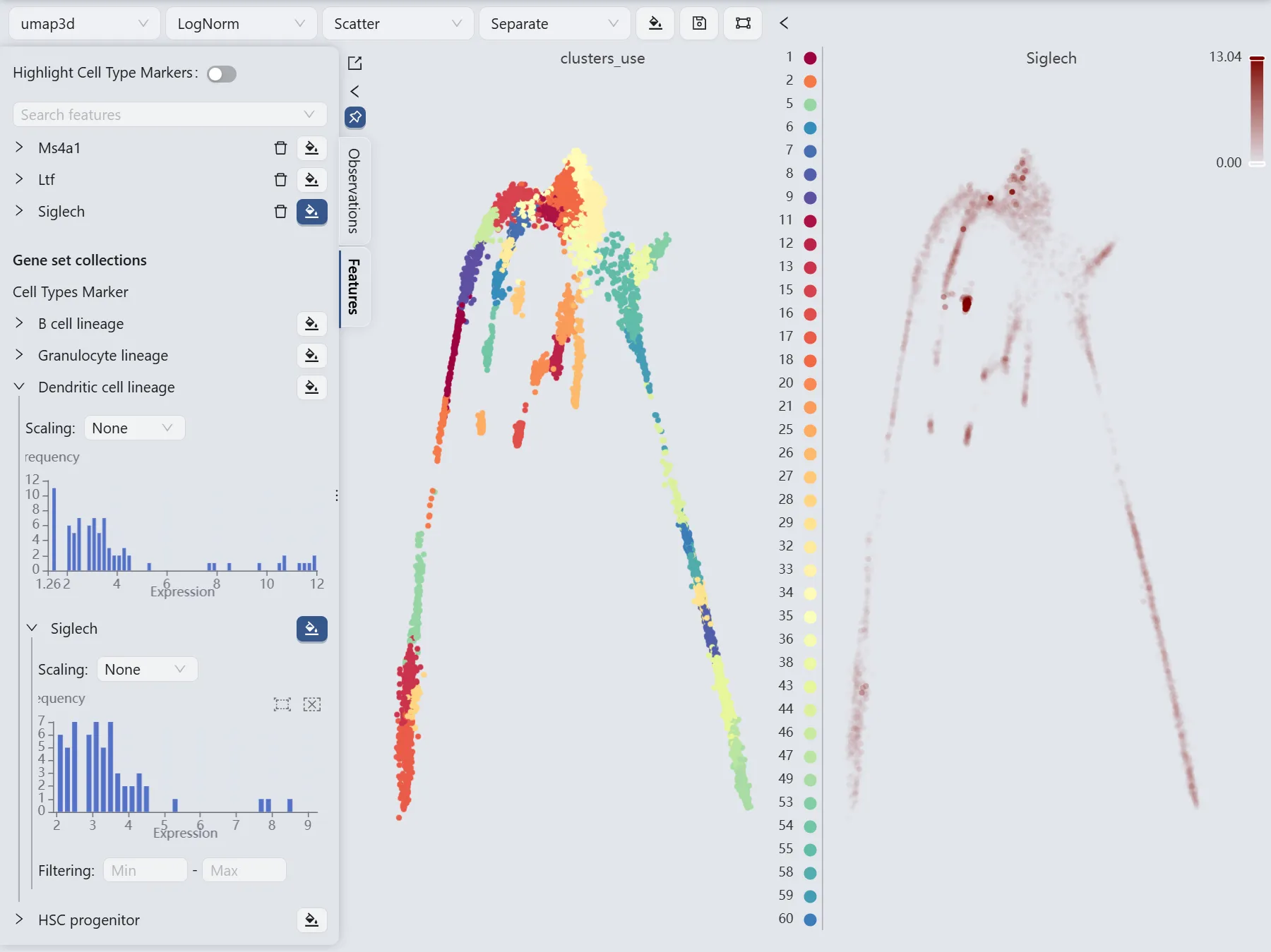
The Siglech gene expression patterns (the right panel) reveal high Siglech expression in cluster 35 and minimal expression in clusters 18 and 27. Based on these expression patterns, we designate cluster 5 as the starting point and clusters 18 and 27 as endpoints for the Slingshot trajectory inference parameters.
Perform trajectory inference analysis for the Siglech gene
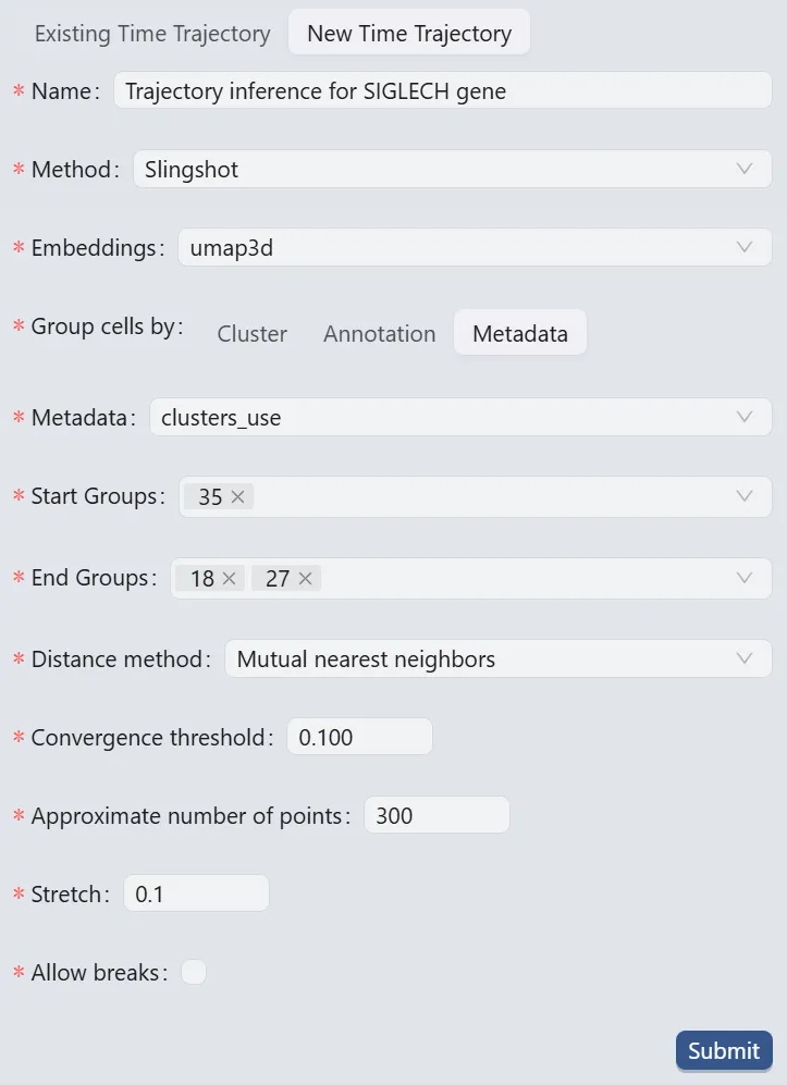
Follow these settings to perform the analysis:
Name:
Trajectory inference for SIGLECH gene. Analysis identifier.Method:
Slingshot. Trajectory inference method used for the analysis.Embeddings:
umap3d. Embedding used for the analysis. In this case, we use the generated embedding from the dataset author.Group cells by:
Metadata. Specifies cell grouping method.Metadata
cluster_use. Metadata field for cell grouping. In this case, we use the clustering analysis result from the dataset author.Start Groups:
35. Initial cluster for the trajectory inference analysis.End Groups:
18,27. Terminal clusters for the trajectory inference analysis.Distance method:
Mutual nearest neighbors. Method for computing inter-cluster distances.Convergence threshold:
0.100. Threshold for change in total distance between cells and curve projections.Approximate number of points:
300. Number of points along trajectory curves.Stretch:
0.1. Curve extrapolation factor beyond endpoints.Allow breaks:
False. Ensures continuous principal curves from origin.
Click the Submit button to create the trajectory inference analysis.
Browse and Visualize Trajectory Inference Analysis Results for the Siglech gene
Once the trajectory inference is completed, the results will be added to the Trajectory Inference Table in the Existing Time Trajectory tab.
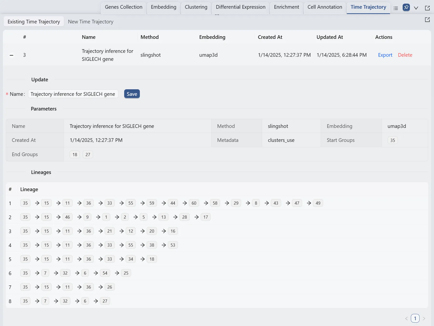
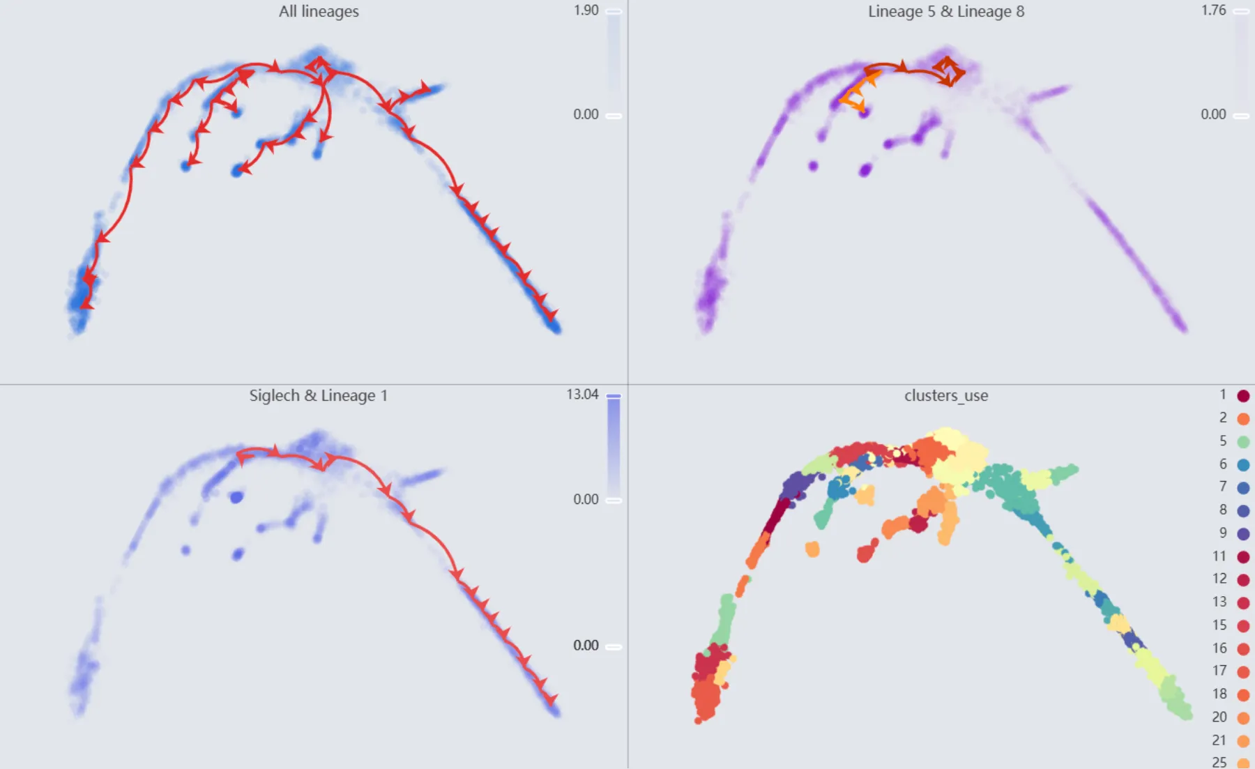
Also, we will display multiple plots to visualize the analysis results. The details of all the plots are:
First plot:
All lineages. Displays the complete trajectory lineage map of the analysis.Second plot:
Lineage 5 & Lineage 8. Shows the developmental pathways from the starting to the ending groups.Third plot:
Siglech & Lineage 1. Illustrates theSiglechgene expression overlay with the representative lineageLineage 1.Fourth plot:
clusters_use. Shows the original clustering result that helped determine the starting and the ending groups.
Trajectory inference for the Cd34 gene
Visualize the Cd34 gene expression
We will observe the expression of the Cd34 gene to manually select the starting and ending points for the Slingshot method parameters.
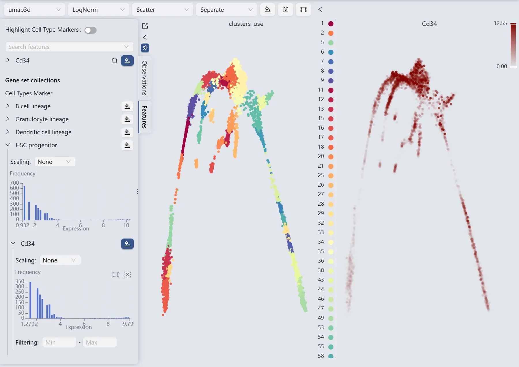
The Cd34 gene expression patterns (the right panel) reveal high Cd34 expression in cluster 34 and minimal expression in clusters 17 and 27. Based on these expression patterns, we designate cluster 5 as the starting point and clusters 17 and 49 as endpoints for the Slingshot trajectory inference parameters.
Additionally, the author's analysis included clusters 27, 25, 16, 26, and 53 as ending groups. Consequently, we will also include these clusters in our ending groups for the comparison between our analysis results with those of the author.
Perform trajectory inference analysis for the Cd34 gene
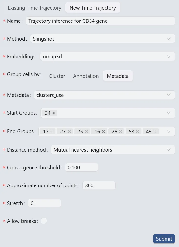
Follow these settings to perform the analysis:
Name:
Trajectory inference for CD34 gene. Analysis identifier.Method:
Slingshot. Trajectory inference method used for the analysis.Embeddings:
umap3d. Embedding used for the analysis. In this case, we use the generated embedding from the dataset author.Group cells by:
Metadata. Specifies cell grouping method.Metadata
cluster_use. Metadata field for cell grouping. In this case, we use the clustering analysis result from the dataset author.Start Groups:
34. Initial cluster for the trajectory inference analysis.End Groups:
17,27,25,16,26,53, and49. Terminal clusters for the trajectory inference analysis.Distance method:
Mutual nearest neighbors. Method for computing inter-cluster distances.Convergence threshold:
0.100. Threshold for change in total distance between cells and curve projections.Approximate number of points:
300. Number of points along trajectory curves.Stretch:
0.1. Curve extrapolation factor beyond endpoints.Allow breaks:
False. Ensures continuous principal curves from origin.
Click the Submit button to create the trajectory inference analysis.
Browse and Visualize Trajectory Inference Analysis Results for the Cd34 gene
Once the trajectory inference is completed, the results will be added to the Trajectory Inference Table in the Existing Time Trajectory tab.
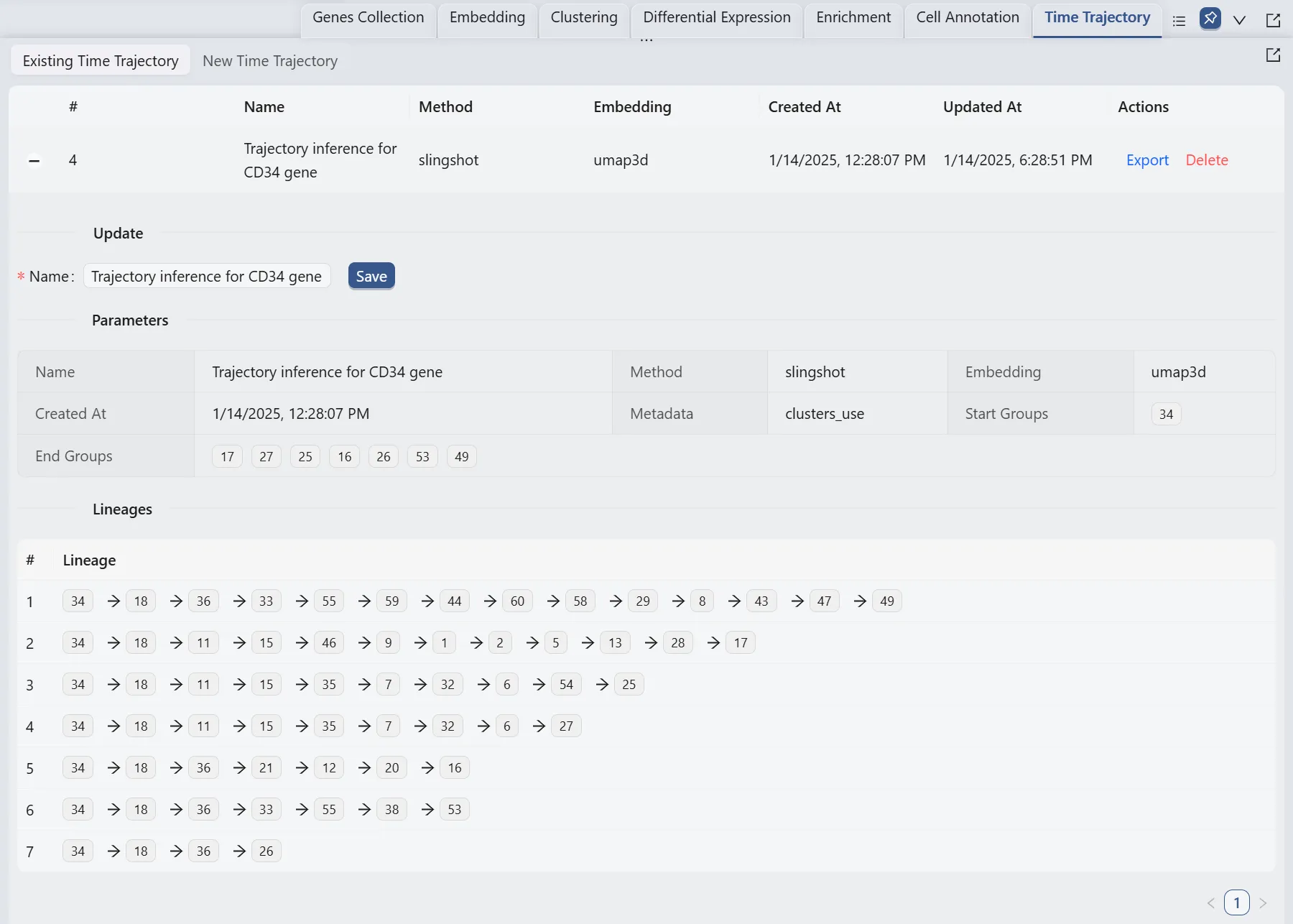
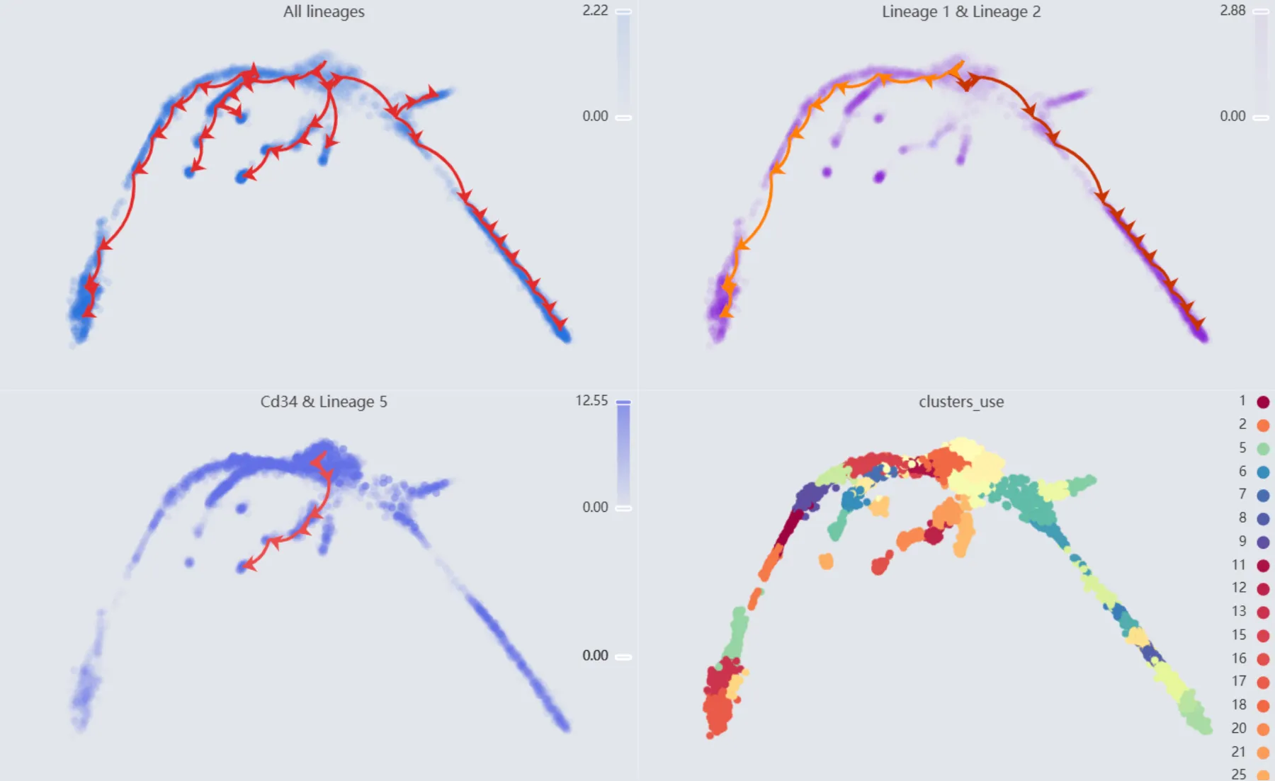
The original study conducted trajectory inference analysis for the Cd34 gene and provided a lineages table for their results.

By comparing the author's lineages table, we can see a perfect concordance between the two analyses.
Finally, we will display multiple plots to visualize the analysis results. The details of all the plots are:
First plot:
All lineages. Displays the complete trajectory lineage map of the analysis.Second plot:
Lineage 1 & Lineage 2. Shows the developmental pathways from the starting to the ending groups.Third plot:
Cd34 & Lineage 5. Illustrates theCd34gene expression overlay with the representative lineageLineage 5.Fourth plot:
clusters_use. Shows the original clustering result that helped determine the starting and the ending groups.
